Backpropagation

Neural network는 categorical classifier에 매우 강력하다. 하지만 크고 복잡한 neural network system에서는 어떻게 gradient를 계산할까.
우리가 이전에 보았던 loss function을 미분하고 graidient를 계산하는 방식은 neural network와 같은 매우 복잡한 모델에서 실현가능하지 못한다. 뿐만 아니라 모듈화 되어있지 않아 중간에 loss function을 바꿀 수도 없다. computer science 관점에서 data structure와 algorithms의 개념을 사용하여 위의 문제를 해겨하며 graident를 계산해보자.

Computational Graphs

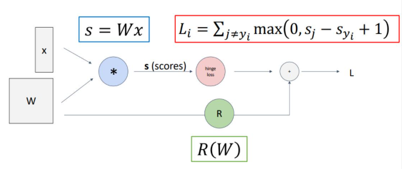
위의 그림은 이전에 보았던 linear classifier model의 loss를 계산하는 과정을 hypothesis function, loss function, regularization term 과정을 뜻하는 각 노드로 나누어 graph로 나타낸 것이다. 앞의 computational graph는 linear classifier를 computational graph로 나타낸 형식적인 graph이지만 모델이 점점 더 커지고 복잡한 형태가 될 수록 이러한 방식은 중요하게 다가올 것이다.

Depp Network (AlexNet)

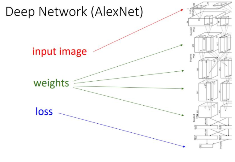위 그림이 나타내는 AlexNet을 보면 많은 layer를 통해 model의 모든 계산 과정이 computational graph를 통해 구조화되고 형식화되어 있다는 볼 수 있따. 간단한 function을 통해 이러한 computational graph를 나타낸보고 backpropagation이라는 과정을 통해 gradient를 계산해 나가는 과정을 살펴볼 것이다.

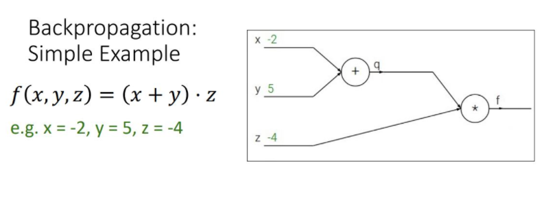
Backpropagation: Simple Example

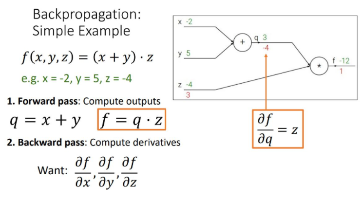
• 1. Forward pass : compute output : 주어진 input값으로 computational graph의 모든 노드를 계산하고 output을 계산한다.
     \(q = x+y, f=q*z\)
     
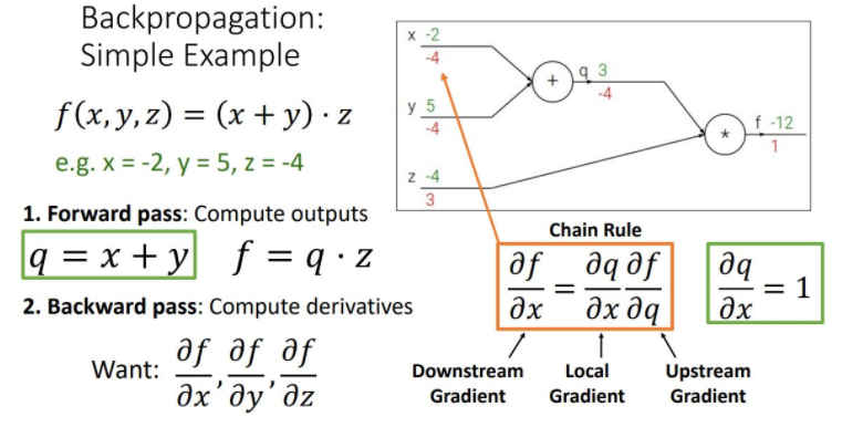
• 1. Backward pass : Compute derivatices : output의 노드부터 전체 functiondls f를 각 노드가 나타내는 함수로 편미분하여 upstream gradient를 만들고, chain rul을 적용시켜 local gradient(현재 노드의 gradient)를 upstream gradient과 곱해주어 상위 노드의 gradient를 계산하는 과정으로 처음 input단의 gradient를 계산해 나가는 방식이다.
• 2_1 : compute local gradient
• 2_2 : compute downstream gradient
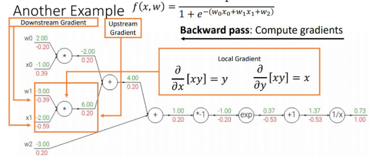
  이러한 backpropagation 과정을 하나의 노드관점에서 나타내면 다음 그림과 같다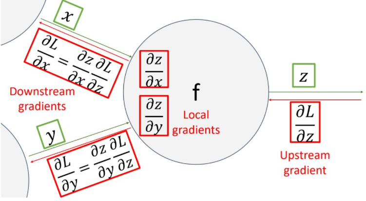
  

이 그림의 핵심은 하나의 노드 입장에서 input변수에 해당하는 gradient(downstream gradient)를 계산하기 위해 upstream gradient와 local gradient를 계산하여 chain rule을 통해 gradient를 곱해준다는 것이다.

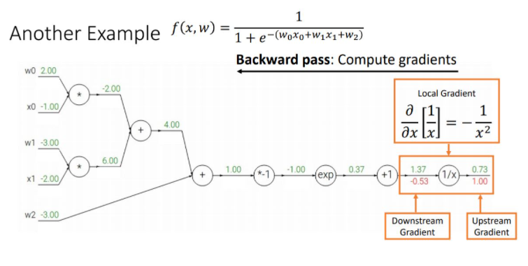
downstream gradient = upstream gradient *local gradient.

\(1 * -(1/1.37^2) = -0.53\)


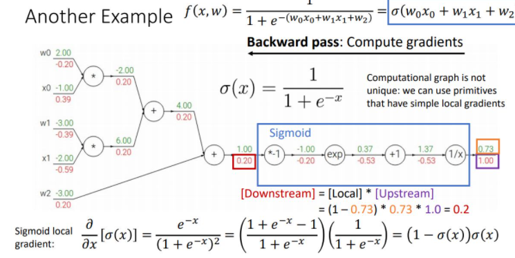
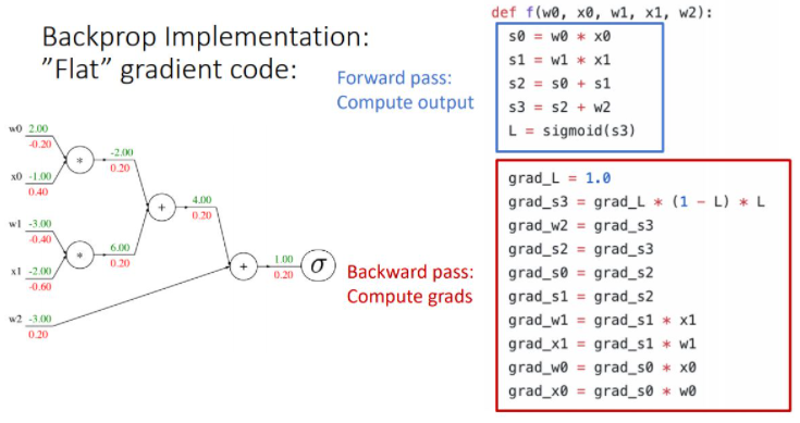
위 그림은 sigmoid function을 통해 좀 더 간편하고 효율적으로 gradient를 꼐산하는 것을 보여준다. 이와같이 computational graph의 최종 loss를 통해 input단의 original parameter들의 gradient를 계산하는 backpropagation과정에서 나타나는 몇개의 패턴을 볼 수 있다.

Patterns in backprop

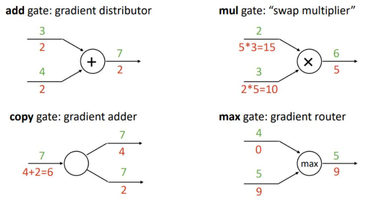
add gate, swap multiplier, gradient adder, gradient router

Backprop with Vectors

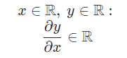
1. where input x is scarlar, output y is scarlar then derivative of y is scarlar
   
   

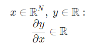
2. where input x is n-dim vector, output y is scarlar then derivative of y is n-dim vector(gradient) 그림 잘못나옴 \(R^N\)

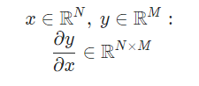
1. where input x is n-dim vector, output is m-dim vector the derivative of y is n by m matrix (jacobian matrix)
   
   

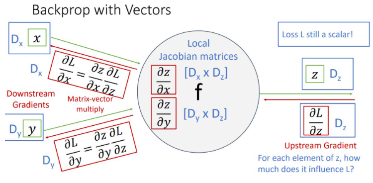
위 그림에서 input x는 x-dim vector이고 input y는 y-dim vector이고 output z는 z-dim vector일때 한 node를 나타낸 것이다. 이때 중요한 것은 output은 vector이지만 loss는 언제나 scalar라는 것이다.

upstream gradient인 ∂L/∂zdms scalar인 loss를 vector z로 편미분한 형태잉기에 derivative는 gradient인 z-dim vector가 된다. 이는 z vector에 각 element가 얼마나 loss에 영향을 미치는가를 나타낸다.
local gradient는 각각 z-dim vector를 x-dim, y-dim vector로 편미분한 형태이기에 derivative은 각각 x by z matrix, y by z matrix인 jacobian matrix가 된다.

마지막으로 downstream gradient는 chain rule을 통해 각각 해당하는 local gradient와 upstream gradient를 곱해주어 계산할 수 있다.

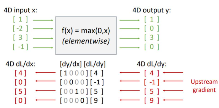
위의 그림처럼 downstream gradient를 구하기위해 local gradient인 ReLU의 x에 대한 도함수 dy/dx matrix(jacobian matrix)와 upstream gradient dL/dy를 곱해준다. 하지만 실질적으로 사용되는 vector들은 high-dimensional vector이기 때문에 jacobian matrix는 매우매우 커져 연산량이 많아지게 되고 매우 sparse해져 비효율적이게 되어 우리는 이러한 jacobian matrix를 대놓고 쓰지 않고 아래 그림과 같은 implicit multiplication을 사용한다.

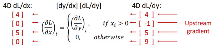
input이 0보다 클때만 pass해서 계산해준다 (?)

이제 input과 output이 vector가 아닌 matrix(혹은 rank가 1 이상인 tensor) 형태일때 backprop을 봐야한다.

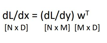
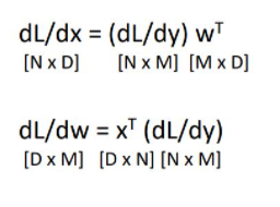
Backprop with matrices

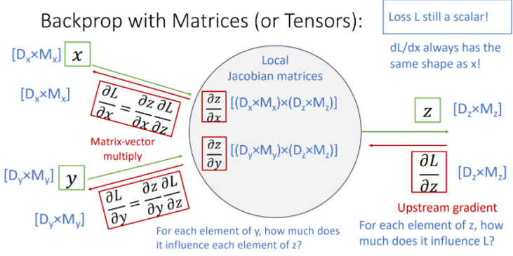
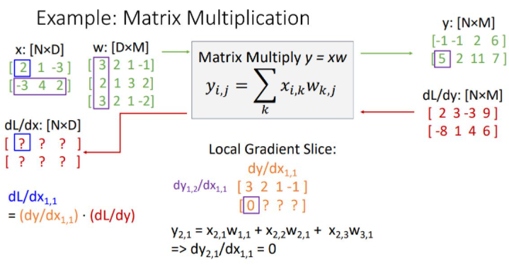
이전과 같은 형태의 form에서 x,y가 matrix form이며 z도 matrix form일때 backprop하는 과정을 보여준다.

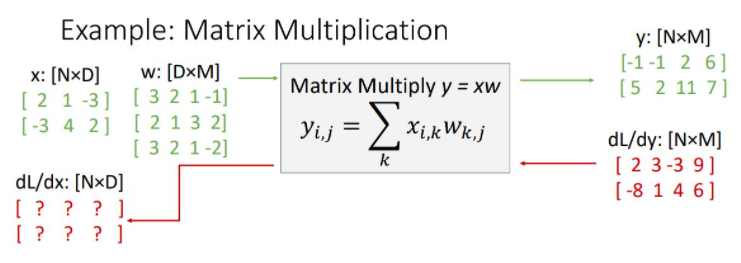
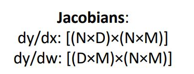
local gradient는 위와같은 형태로 매우 큰 jacobian matrix가 된다. 이전에 vector에 대한 jacobian도 감당할 수 없는데 얘는 정말 크다. 그래서 우리는 jacobian matrix 전체를 multiplication해주어 downstream gradient를 구하는 것이 아니라 jacobbian matrix를 implicitly 사용하여 element 관점에서 하나하나 구해보려고 함

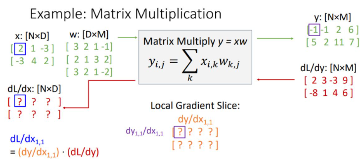
x에 대한 downstream gradient인 dL/dx는 당연하게도 x의 form과 똑같다. (N by D) 이런 dL/dx에서 첫번째 element를 구해보자(위 그림의 파란박스)

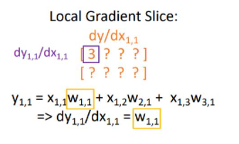
위의 그림과 같이 Local Gradient Slice를 구할 수 있다. dy1,1/dx1,1 = w1,2(3)이다.

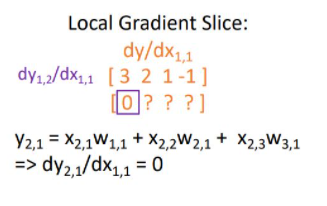
이런식으로 dy/dx1,1을 채워나간다.

위의 그림에서 볼수 있듯이 두번째 열에는 모두 zero vector가 된다. 왜냐면 y의 2번째 열을 만드는 데에는 x1,1이 관여하지 않았고 그래서 편미분하면 다 상수처리되어서 0이된다.

사실 local gradient와 upstream gradient의 matrix multiplication을 하기위해선 아래 그림과 같이 두 matrix의 순서를 바꾸고 upstream gradient를 transpose히켜줘야한다.